⏱ 14 min read
Introduction
Systems Modeling Language (SysML) is the standard language for model-based systems engineering. One of its most powerful capabilities — and one of the least understood — is its integration with Modelica for simulation. SysML defines the structure, constraints, and relationships of a system. Modelica provides the mathematical engine that makes those models executable. Together, they allow engineers to move from "this is what our system looks like" to "this is how our system behaves" without leaving the modeling environment.

This article walks through a complete set of Modelica simulation examples built in Sparx Enterprise Architect. Each example demonstrates different SysML constructs — block definition diagrams, parametric diagrams, constraint blocks, value types, port types, and flow specifications — applied to real physics and engineering problems. The examples progress from simple (drawing a circle) to complex (coupled fluid tanks with PID control), giving you a practical toolkit for SysML-Modelica integration.
Everything shown here is modeled using standard SysML notation with the Modelica profile in Sparx EA. No custom code, no external tools — just the model, the simulation engine, and the results. Sparx EA best practices
Model Overview and Package Structure
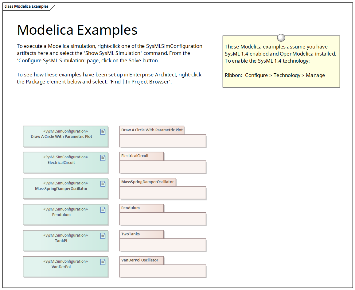
The package structure follows good SysML modeling practice: a root package "Modelica Examples" contains seven self-contained example packages, each demonstrating different modeling concepts. The "CommonlyUsedTypes" and "PrimitiveValueTypes" packages provide shared value type libraries that are imported across all examples. This modular structure means each example is independently understandable while sharing a common type foundation.
The seven examples — Draw a Circle, Electrical Circuit, Mass-Spring-Damper Oscillator, Pendulum, Two Tanks, Van der Pol Oscillator, and the shared type libraries — cover a remarkable breadth of engineering domains: geometry, electronics, mechanical dynamics, multi-body physics, fluid dynamics, and nonlinear control theory. Each one uses different SysML diagram types and Modelica constructs, making the collection a comprehensive reference for practitioners.
Foundations: Value Types and Primitives
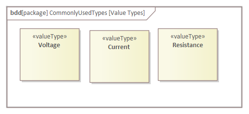
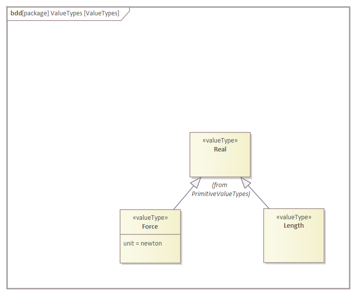
Every simulation model needs a consistent type system. The CommonlyUsedTypes package defines the SysML value types that map to Modelica primitive types: Real (with units like meters, seconds, kilograms, radians), Integer, Boolean, and String. Each value type carries unit and dimension information — not just "a number" but "a number in meters per second squared." This dimensional consistency is what prevents unit mismatch errors that plague spreadsheet-based engineering calculations.
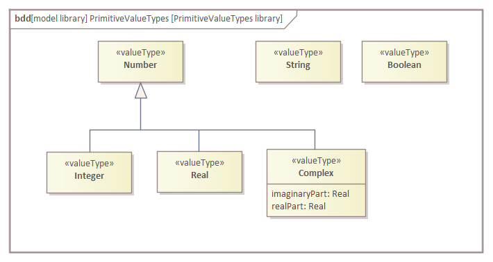
The PrimitiveValueTypes library goes deeper, defining the base types that Modelica needs to compile and execute simulations. These are the building blocks that constraint expressions, port types, and block properties reference. Having them in a shared library package means every example in the model uses exactly the same type definitions — a small detail that prevents a large category of modeling errors.
Drawing a Circle: Parametric Constraints in Action
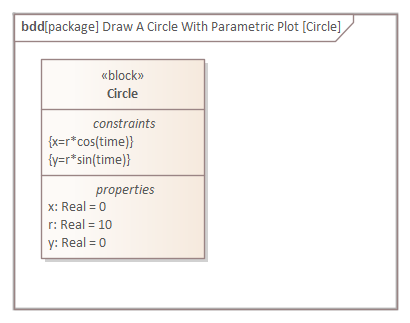
This is the simplest example and the best starting point. The model uses a single SysML constraint block with the equation x² + y² = r² to generate a circle. The parametric diagram connects a radius value to the constraint, and the Modelica solver computes the x and y coordinates over a sweep. The result is a parametric plot — a circle drawn entirely by the simulation engine from a mathematical constraint.
Why does this matter? Because it demonstrates the core SysML-Modelica workflow in its purest form: define a constraint in SysML, bind parameters to it, run the Modelica simulation, and get a result. Every subsequent example follows this same pattern — just with more complex physics.
Electrical Circuit: A Complete SysML-Modelica Example
The Electrical Circuit example is the most comprehensive single example in the collection. It demonstrates package imports, composite types, constraint blocks, and a fully wired circuit model — all using standard SysML constructs.
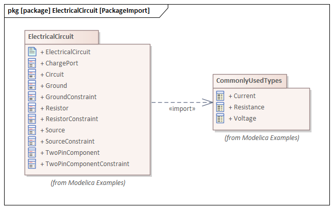
The package import diagram shows how the model references the Modelica Standard Library. Rather than defining resistor and capacitor physics from scratch, the model imports standard Modelica.Electrical.Analog components. This is the SysML equivalent of "import" in code — it gives the model access to pre-validated, tested component libraries. In Sparx EA, these imports are managed through SysML package import relationships that the Modelica code generator resolves automatically. free Sparx EA maturity assessment
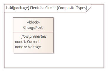
The composite types diagram defines the blocks that represent circuit components. Each block — Resistor, Capacitor, VoltageSource, Ground — carries properties (resistance in Ohms, capacitance in Farads, voltage in Volts) and ports (electrical pins). The properties are typed using the value types from the shared library. The ports define the connection points where components interface with each other. This is standard SysML block definition — the same notation you would use for any system, but here the blocks happen to represent electrical components. modeling integration architecture with ArchiMate
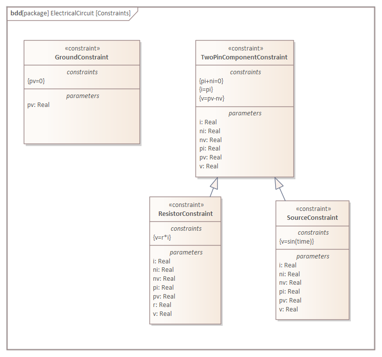
The constraint blocks are where the physics lives. Each constraint block encapsulates a mathematical relationship: Ohm's law (V = IR), the capacitor equation (I = C × dV/dt), and Kirchhoff's current and voltage laws. These are SysML constraint blocks — not code, not comments, but formal model elements with typed parameters that the Modelica solver uses to compute the simulation. When the model is executed, these constraints become the differential equations that Modelica integrates over time. enterprise cloud architecture patterns
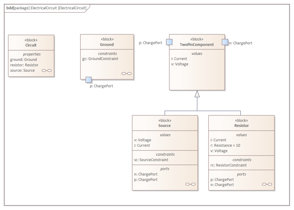
The internal block diagram is the payoff. It shows the complete circuit: components instantiated from the block definitions, wired together through their electrical ports, with property values assigned. This is exactly what a circuit schematic shows — but in SysML notation, with full traceability to the block definitions, constraint equations, and value types. When you run the Modelica simulation, the solver computes voltages and currents at every node over time, producing time-series plots that validate the circuit behavior.
Mass-Spring-Damper Oscillator
The Mass-Spring-Damper (MSD) oscillator is the "hello world" of mechanical dynamics. A mass attached to a spring and damper, pulled and released, oscillates with decreasing amplitude until friction dissipates all energy. The SysML model captures this physics completely.
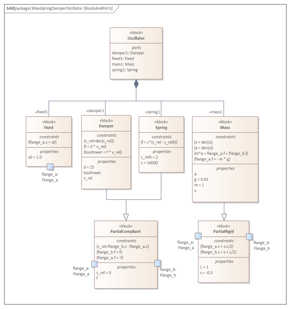
The block definition diagram defines four blocks: Mass, Spring, Damper, and Fixed (the anchor point). Each block has mechanical translational ports — interfaces that carry force and velocity signals. The Spring block has a stiffness property (N/m), the Damper has a damping coefficient (N·s/m), and the Mass has a mass property (kg). These are physical properties, not abstract attributes — each one has units, and those units are enforced by the value type system.
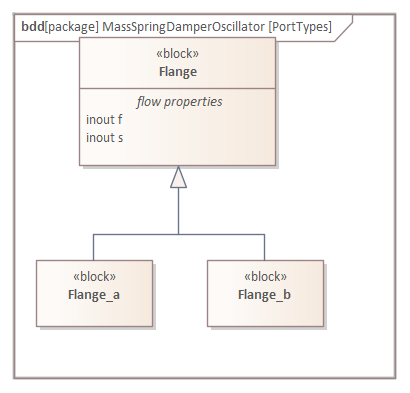
The port types diagram defines what flows through the connections between blocks. A mechanical translational port carries two conjugate variables: force and velocity. When two ports are connected, force is equalized and velocities are coupled. This is the SysML equivalent of Modelica's connector concept — a typed interface that enforces physical consistency at every connection point.
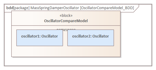
The comparison model is particularly valuable for engineering analysis. By creating multiple instances of the oscillator with different parameter values — different spring stiffness, different damping coefficients — engineers can run parameter sweeps and compare behaviors. The BDD shows the comparison structure: same block types, different property values, different simulation results. This is model-based engineering in action: change a parameter, re-run the simulation, compare the outcome.
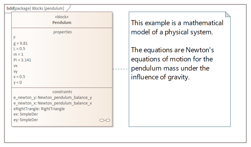
Pendulum: Multi-Body Dynamics
The Pendulum example steps up to rotational dynamics and gravitational forces — a system with nonlinear behavior that cannot be solved analytically for large angles.
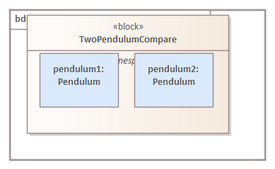
The two-pendulum comparison shows pendulums started from different angles. For small angles, the motion is nearly sinusoidal (the linear approximation holds). For large angles, the motion becomes visibly nonlinear — the period increases and the waveform distorts. This is exactly the kind of insight that simulation provides and hand calculation cannot: the quantitative boundary where linear assumptions break down.
The value types for the pendulum include angular displacement (radians), angular velocity (rad/s), torque (N·m), moment of inertia (kg·m²), and gravitational acceleration (m/s²). Each type carries its SI unit, ensuring dimensional consistency throughout the constraint equations. If you accidentally wire a force where a torque is expected, the type system catches it before simulation.
Two Tanks: Fluid Dynamics and Control
The Two Tanks example is the most engineering-realistic model in the collection. Two fluid tanks connected by pipes, with flow rates governed by pressure differences, and PID controllers managing fluid levels. This is a classic process control problem.
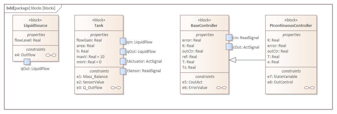
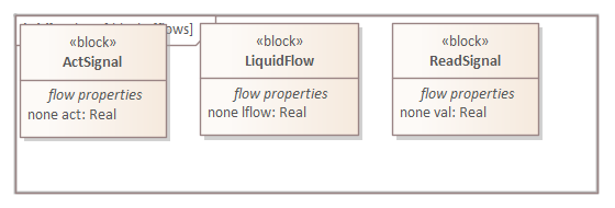
The flow specification diagram defines what flows between tanks and pipes: mass flow rate (kg/s), pressure (Pa), and temperature (K). This is a multi-variable flow — not just "fluid goes from A to B" but a physically complete description of the fluid state at every connection point. SysML flow ports with flow specifications are the right abstraction for this kind of continuous physical interaction.
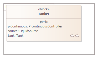
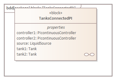
The connected tanks parametric diagram shows the full control architecture: Tank 1's level is controlled by Valve 1, Tank 2's level is controlled by Valve 2, but fluid flowing from Tank 1 to Tank 2 means the controllers are coupled. When Controller 1 opens Valve 1 to fill Tank 1, the increased pressure drives more fluid into Tank 2, causing Controller 2 to react. This cross-coupling is exactly what makes real process control challenging — and what the simulation reveals.
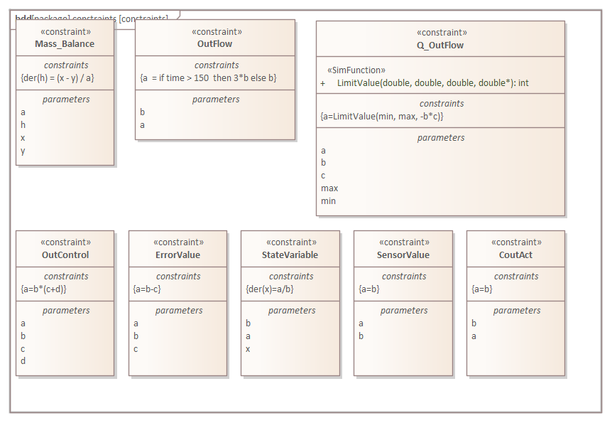
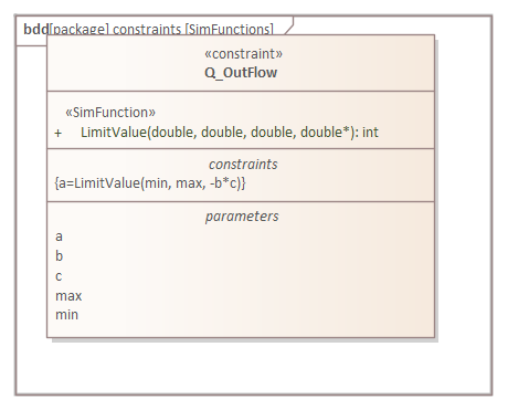
The simulation functions define the test scenarios: step changes in setpoint (sudden demand for a different level), ramp inputs (gradually changing targets), and disturbance signals (simulating unexpected inflows or outflows). These are the stimuli that exercise the control system and reveal its dynamic behavior — overshoot, settling time, steady-state error, and stability margins.
Van der Pol Oscillator: Nonlinear Dynamics
The Van der Pol oscillator is a classic nonlinear dynamics problem that produces self-sustaining oscillations — a limit cycle. Unlike the linear MSD oscillator where amplitude decays to zero, the Van der Pol system settles into a stable periodic orbit regardless of initial conditions.
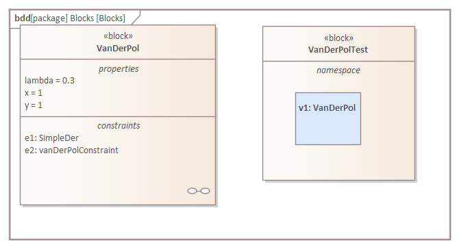
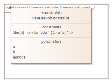
The constraint block encapsulates the Van der Pol equations: dx/dt = y and dy/dt = μ(1-x²)y - x. The parameter μ controls the nonlinearity strength. When μ is small, the system behaves almost linearly. As μ increases, the oscillation becomes increasingly "relaxation-like" — sharp transitions between slow and fast phases. By varying μ in the SysML model and running simulations, engineers can explore this bifurcation behavior systematically.
This example demonstrates that SysML-Modelica integration is not limited to "engineering" problems in the traditional sense. Any system governed by differential equations — biological systems, economic models, epidemiological dynamics — can be modeled and simulated using these same patterns. integration architecture diagram
SysML Modeling Patterns Demonstrated
Across the seven examples, several reusable SysML modeling patterns emerge that are applicable to any domain.
Pattern 1: Shared Type Libraries. Every example imports from CommonlyUsedTypes and PrimitiveValueTypes. This pattern — defining value types with units in a shared package and importing them across models — prevents unit inconsistencies and enables model composition. When you combine an electrical subsystem with a mechanical subsystem, both use the same definition of "Newton" and "meter."
Pattern 2: Block-Port-Connector Architecture. Components are defined as blocks, their interfaces as ports, and their physical interactions as connectors. This three-layer pattern scales from a simple spring to a complex process control system. The port types enforce interface compatibility: you cannot connect an electrical port to a fluid port.
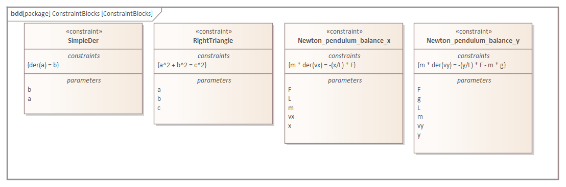
Pattern 3: Constraint Blocks for Physics. Mathematical relationships are modeled as SysML constraint blocks, not as code annotations or documentation. This makes the physics first-class model elements that can be validated, traced, and reused. The circle equation, Ohm's law, Newton's second law, and the PID controller algorithm are all constraint blocks.
Pattern 4: Parametric Diagrams for Binding. Parametric diagrams connect constraint blocks to block properties, binding abstract equations to concrete parameter values. This separation — constraints define relationships, parametric diagrams bind values — makes it easy to reuse the same physics with different parameter sets.
Pattern 5: Comparison Models for Analysis. The oscillator comparison and two-pendulum comparison models show how to create variant configurations for parameter studies. Same block types, different property values, compared simulation results. This is the foundation of model-based trade studies and design space exploration.
Pattern 6: Package Import for Library Reuse. The electrical circuit's import of the Modelica Standard Library components demonstrates how to leverage existing validated component libraries rather than building everything from scratch. This is the SysML equivalent of "don't reinvent the wheel" — use the community's tested components and focus your modeling effort on what is novel about your system.
Conclusion
These seven Modelica examples demonstrate that SysML is not just a documentation language — it is a systems engineering workbench that connects structure to behavior through simulation. Every diagram shown in this article was created in Sparx Enterprise Architect using standard SysML notation with the Modelica profile. The models are executable: change a parameter value, press simulate, and see the results.
For systems engineers looking to move beyond static diagrams into model-based systems engineering with simulation, the SysML-Modelica combination is the industry standard path. The patterns demonstrated here — shared type libraries, block-port-connector architecture, constraint blocks, parametric binding, comparison models, and library reuse — are applicable to any engineering domain from aerospace to automotive to medical devices.
For expert guidance on SysML modeling and simulation, explore our SysML training, Sparx EA training, and consulting services. Get in touch.
Frequently Asked Questions
What is Sparx Enterprise Architect used for?
Sparx Enterprise Architect (Sparx EA) is a comprehensive UML, ArchiMate, BPMN, and SysML modeling tool used for enterprise architecture, software design, requirements management, and system modeling. It supports the full architecture lifecycle from strategy through implementation.
How does Sparx EA support ArchiMate modeling?
Sparx EA natively supports ArchiMate 3.x notation through built-in MDG Technology. Architects can model all three ArchiMate layers, create viewpoints, add tagged values, trace relationships across elements, and publish HTML reports — making it one of the most popular tools for enterprise ArchiMate modeling.
What are the benefits of a centralised Sparx EA repository?
A centralised SQL Server or PostgreSQL repository enables concurrent multi-user access, package-level security, version baselines, and governance controls. It transforms Sparx EA from an individual diagramming tool into an organisation-wide architecture knowledge base.